Case Studies
Below are a number of case studies conducted
using PARAM. Most of them are parametric variants of
case studies from the PRISM homepage.
For the SPIN 2010 case studies [CalinCDHZ10],
we consider a scenario where each process is
assigned a different scheduler, which has incomplete information about
the state of the other processes. To
simulate the incompleteness of informations, we encode nondeterminism
into parametric probabilistic choice. Then, we use PARAM
to compute a parametric reachability probability and lateron use
a nonlinear optimisation program (currently Matlab) to
compute the optimal reachability probability under the restricted
scheduler class. In the first notion we introduced in our SPIN 2010
paper, there are distributed schedulers
which still have behaviour which one would want to exclude for some
models. Because of this, we extended our notion to strong
schedulers, where we restrict the possible behaviours further. The
modelling mechanism we use are input/output interactive chains where
there is a distinction between input (labelled with "?") and
output (labelled with "!") actions. For these models,
PARAM was run on a 3GHz computer with 1GB of
memory, while Matlab was run on a computer with two 1.2Ghz
processors and 2GB of memory. The models from SPIN 2010 are available
on request.
- Randomised Consensus Protocol (NFM 2011)
- Crowds Protocol (SPIN 2009/STTT/CAV 2010)
- Zeroconf (SPIN 2009/STTT)
- Cyclic Polling Server (SPIN 2009/STTT)
- Randomised Mutual Exclusion (SPIN 2009/STTT)
- Bounded Retransmission Protocol (SPIN 2009/STTT)
- Mastermind (SPIN 2010)
- Dining Cryptographers (SPIN 2010)
- Randomized Scheduler Example (SPIN 2010)
- Monty Hall (Presentation of Master's thesis of Georgel Calin)
Randomised Consensus Protocol (NFM 2011)
We applied PARAM 2.0 α on a randomised consensus shared coin
protocol by Aspnes and Herlihy [AspnesH90], based on an existing
PRISM model [KwiatkowskaNS01]. In this case study, there are
N processes sharing a counter c, which initially has the
value 0. In addition, a value K is fixed for the protocol. Each
process i decides to either decrement the counter with probability
pi or to increment it with probability 1 - pi. In contrast to
the original PRISM, we do not fix the pi to 1/2,
but use them as parameters of the model. After writing the counter,
the process
reads the value again and checks whether c ≤ -KN or c ≥
KN. In the first case, the process votes 1, in the second it votes
2. In both cases, the process stops afterwards. If neither of the
two cases hold, the process continues its execution. As all processes
which have not yet voted try to access the counter at the same time,
there is a nondeterministic choice on the access order.
A probabilistic formula
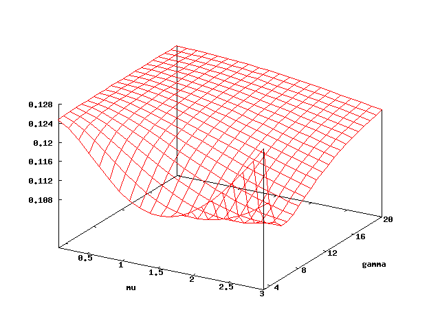
As the first property, we ask whether for each execution of the protocol the probability that all processes finally terminate with a vote of 2 is at least (K-1)/(2K). With appropriate atomic propositions finished and allCoinsEqualTwo, this property can be expressed as P≥(K-1)/(2K)(true U (finished ∧ allCoinsEqualTwo)). For the case N=2 and K=2, we give results in the figure below.
The leftmost part of the figure provides the minimal probabilities among all schedulers that all processes terminate with a vote of 2, depending on the parameters pi. With decreasing pi, the probability that all processes vote 2 increases, since it becomes more likely that a process increases the counter and thus also the chance that finally c ≥ KN holds. The plot is symmetric, because both processes are independent and have an identical structure.
On the right part of the figure, we give an overview which schedulers are optimal for which parameter values. Here, boxes labelled with the same number share the same minimising scheduler. In case p1 < p2, to obtain the minimal probability the nondeterminism must be resolved such that the first process is activated if it has not yet voted. Doing so maximises the probability that we have c ≤ -KN before c ≥ KN, and in turn minimises the probability that both processes vote 2. For p1 > p2, the second process must be preferred.
In the middle part of the figure, we give the truth values of the formula. Cyan boxes correspond to regions where the property holds, whereas in red boxes it does not hold. In white areas, the truth value is undecided. To keep the white areas viewable, we chose a rather high tolerance of 0.15. The truth value decided is as expected by inspecting the plot on the left part of the figure, except for the white boxes along the diagonal of the figure. In the white boxes enclosed by the cyan area, the property indeed holds, while in the white areas surrounded by the red area, it does not hold. The reason that these areas remain undecided is that the minimising scheduler changes at the diagonals, as discussed in the previous paragraph. If the optimal scheduler in a box is not constant for the region considered, we have to split it. Because the optimal scheduler always changes at the diagonals, there are always some white boxes remaining.
A Reward Formula
As a second property, we ask whether the expected number of steps until all processes have voted is above 25, expressed as R>25(F finished). Results are given in the figure below. On the left part, we give the expected number of steps. This highest value is at pi = 1/2. Intuitively, in this case the counter does not have a tendency of drifting to either side, and is likely to stay near 0 for a longer time. Again, white boxes surrounded by boxes of the same colour are those regions in which the minimising scheduler is not constant. We see from the right part of the figure that this happens along four axes. For some values of the parameters, the minimising scheduler is not always the one which always prioritises one of the processes. Instead, it may be necessary to schedule the first process, then the second again, etc. As we can see, this leads to a number of eight different schedulers to be considered for the considered variable ranges.
Runtime
In the table below, we give the runtime of our tool (on an Intel Core 2 Duo P9600 with 2.66 GHz running on Linux) for two processes and different constants K. Column "States" contains the number of states. The columns labelled with "Until" contain results of the first property while those labelled with "Reward" contain those of the second. Columns labelled with "min" contain just the time to compute the minimal values whereas those labelled with "truth" also include the time to compare this value against the bound of the formula. For all analyses, we chose a tolerance of "ε=0.05". The time is given in seconds, and "-" indicates that the analyses did not terminate within 90 minutes.
| K | States | Until | Reward | ||
|---|---|---|---|---|---|
| min | truth | min | truth | ||
| 2 | 272 | 4.7 | 22.8 | 287.8 | 944.7 |
| 3 | 400 | 13.7 | 56.7 | 4610.1 | - |
| 4 | 528 | 31.7 | 116.1 | - | - |
| 5 | 656 | 65.5 | 215.2 | - | - |
| 6 | 784 | 123.4 | 374.6 | - | - |
| 7 | 912 | 272.6 | 657.4 | - | - |
As we see, the performance drops quickly with a growing number of states. For reward-based properties, the performance is worse than for unbounded until. These analyses are more complex, as rewards have to be taken into account, and weak bisimulation can not be applied for minimisation of the induced models. In addition, a larger number of different schedulers has to be considered to obtain minimal values, which also increases the analysis time. We are however optimistic that we will be able to improve these figures, using a more advanced implementation.
- model file
- unbounded until property file (min)
- unbounded until property file (truth)
- accumulated reward property file (min)
- accumulated reward property file (truth)
Crowds Protocol (SPIN 2009/STTT/CAV 2010)
The intention of the Crowds protocol [ReiterR98] is to protect the anonymity of Internet users. The protocol hides each user's communications via random routing. Assume that we have N honest Crowd members, and M dishonest members. Moreover, assume that there are R different path reformulates. The model is a parametric Markov chain with two parameters of the model:
- B=M/(M+N): probability that a Crowd member is untrustworthy
- P: probability that a member forwards the package to a random selected receiver.
With
probability 1-P a crowd member delivers the message to the receiver directly.
We consider the probability that the actual sender was observed more
than any other one by the untrustworthy members. For various N and
R values, the table below summarises the time needed for
computing the function representing this probability, with and without
the weak bisimulation optimisation. With "Build(s)" we denote
the time needed to construct the model for the analysis from the high
level PRISM model. The columns "Elim.(s)"
state the time needed for the state elimination part of the
analysis. "Mem(MB)" gives the memory usage. When applying
bisimulation minimization, "Lump(s)" denotes the time needed
for computing the quotient. For entries marked by "-", the
analysis did not terminate within one hour.
In the last column we evaluate the
probability for M=N/5 (thus B=1/6) and P=0.8.
An interesting observation is that for several table entries
the weak bisimulation quotient has the same size for the same R, but
different probabilities. We also checked that the graph structure was
the same in these cases. The reason for this is that the other
parameter N has only an effect on the transition probabilities of
the quotient and not its underlying graph.
From the table we also see that for this case study the usage of bisimilation helped to speed up the analysis very much. For the N and R considered, the speedup was in the range of about 10 for N=5, R=7 to factor such that the time for the state elimination was negligible, as for N=15, R=3. Also, the time for the bisimulation minimization itself did not take longer than 26 seconds. Using bisimulation minization, we are able to handle models with several hundred thousands of states.
| N | R | Build (s) | no bisimulation | weak bisimulation | Result | |||||||
|---|---|---|---|---|---|---|---|---|---|---|---|---|
| States | Trans. | Elim. (s) | Mem (MB) | States | Trans. | Lump (s) | Elim. (s) | Mem (MB) | ||||
| 5 | 3 | 3 | 1192 | 1982 | 4 | 3 | 33 | 62 | 0 | 0 | 2 | 0.3129 |
| 5 | 5 | 3 | 8617 | 14701 | 57 | 5 | 127 | 257 | 0 | 5 | 6 | 0.3840 |
| 5 | 7 | 5 | 37169 | 64219 | 1878 | 13 | 353 | 732 | 1 | 181 | 15 | 0.4627 |
| 10 | 3 | 3 | 6552 | 14857 | 132 | 4 | 33 | 62 | 0 | 0 | 5 | 0.2540 |
| 10 | 5 | 7 | 111098 | 258441 | 1670 | 40 | 127 | 257 | 2 | 6 | 51 | 0.3159 |
| 10 | 7 | 47 | 989309 | 2332513 | - | - | 367 | 763 | 26 | 259 | 441 | 0.4062 |
| 15 | 3 | 4 | 19192 | 55132 | 504 | 10 | 33 | 62 | 0 | 0 | 12 | 0.2352 |
| 15 | 5 | 31 | 591455 | 1739356 | - | - | 127 | 257 | 14 | 7 | 305 | 0.2933 |
| 20 | 3 | 8 | 42298 | 146807 | 2044 | 22 | 33 | 63 | 1 | 0 | 26 | 0.2260 |
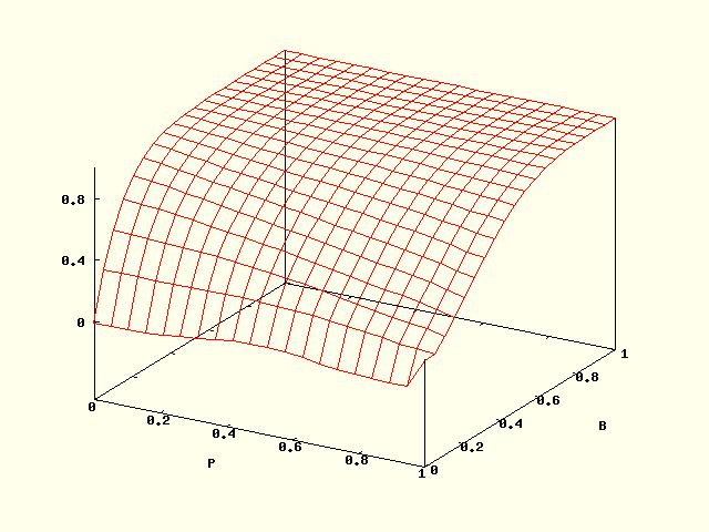
In the figure below, we give the plot for N=5, R=7. Observe that this probability increases with the number of dishonest members M, which is due to the fact that the dishonest members share their local information. On the contrary, this probability decreases with P. The reason is that each router forwards the message randomly with probability P. Thus with increasing P the probability that the untrustworthy member can identify the real sender is then decreased.
Zeroconf (SPIN 2009/STTT)
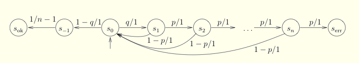
Zeroconf allows the installation and operation of a network in the most simple way. When a new host joins the network, it randomly selects an address among the K=65024 possible ones. With m hosts in the network, the collision probability is q=m/K. The host asks other hosts whether they are using this address. If a collision occurs, the host tries to detect this by waiting for an answer. The probability that the host gets not answer in case of collision is p, in which case he repeats the question. If after n tries the host got no answer, the host will erroneously consider the chosen address as valid. A sketch of the model is depicted in the figure above. We consider the expected number of tries till either the IP address is selected correctly or erroneously, so that the set of target states is B={ok,err}. For n=140, the plot of this function is depicted below.
The expected number of tests till termination increases with both the collision probability as well as the probability that a collision is not detected. Bisimulation optimisation was not of any use, as the quotient equals the original model. For n=140, the analysis took 64 seconds and 50 MB of memory.
Cyclic Polling Server (SPIN 2009/STTT)
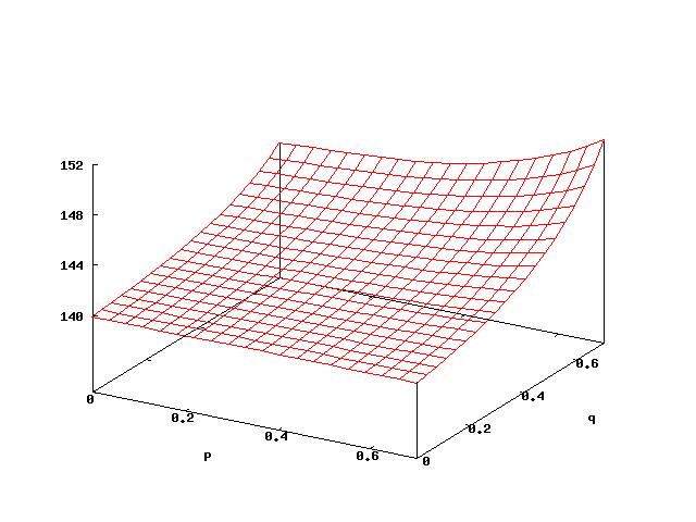
The cyclic polling server [IbeT90] consists of a number of N stations which are handled by the polling server. Process i is allowed to send a job to the server if he owns the token, circulating around the stations in a round robin manner. This model is a parametric continuous-time Markov chain, but we can apply our algorithm on the embedded discrete-time parametric Markov chain, which has the same reachability probability. We have two parameters: the service rate mu and gamma is the rate to move the token. Both are assumed to be exponentially distributed. Each station generates a new request with rate lambda = mu / N. Initially the token is at state 1. We consider the probability p that station 1 will be served before any other one. The table below summarises performance for different N. The last column corresponds to the evaluation mu=1, gamma=200.
| N | Build (s) | no bisimulation | weak bisimulation | Result | |||||||
|---|---|---|---|---|---|---|---|---|---|---|---|
| States | Trans. | Elim. (s) | Mem (MB) | States | Trans. | Lump (s) | Elim. (s) | Mem (MB) | |||
| 4 | 1 | 66 | 192 | 1 | 2 | 13 | 36 | 0 | 0 | 3 | 0.2500 |
| 5 | 1 | 162 | 560 | 2 | 2 | 16 | 46 | 0 | 0 | 3 | 0.2000 |
| 6 | 1 | 386 | 1536 | 10 | 2 | 19 | 58 | 0 | 0 | 2 | 0.1667 |
| 7 | 1 | 898 | 4032 | 41 | 3 | 22 | 68 | 0 | 0 | 3 | 0.1429 |
| 8 | 1 | 2050 | 10240 | 150 | 4 | 25 | 79 | 0 | 1 | 4 | 0.1250 |
| 9 | 2 | 4610 | 25344 | 733 | 6 | 28 | 91 | 0 | 1 | 6 | 0.1111 |
On figure below a plot for N=8 is given. We have several interesting observations. If mu is greater than approximately 1.5, p first decreases and then increases with gamma. The mean time of the token staying in state 1 is 1 / gamma. With increasing gamma, it is more probable that the token pasts to the next station before station 1 sends the request. At some point however (approximated gamma=6), p increases again as the token moves faster around the stations. For small mu the probability p is always increasing. The reason for this is that the arrival rate lambda = mu / N is very small, which means also that the token moves faster. Now we fix gamma to be greater than 6. Then, p decreases with mu, as increasing mu implies also a larger lambda, which means that all other states become more competitive. However, for small gamma we observe that mu increases later again: in this case station 1 has a higher probability of catching the token initially at this station. Also in this model, bisimulation has quite a large effect on the time needed for the analysis.
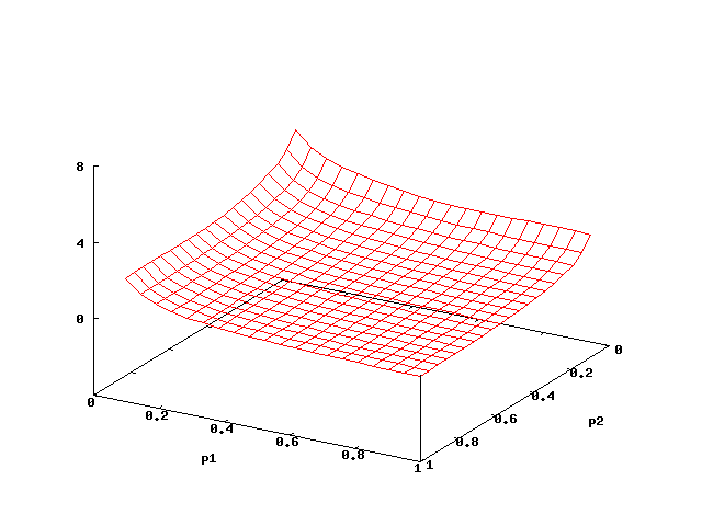
Randomised Mutual Exclusion (SPIN 2009/STTT)
In the randomised mutual exclusion protocol [PnueliZ86] several processes try to enter a critical section. We consider the protocol with two processes i=1,2. Process i tries to enter the critical section with probability pi, and with probability 1-pi, it waits until the next possibility to enter and tries again. The model is a PMRM with parameters pi. A reward with value 1 is assigned to each transition corresponding to the probabilistic branching pi and 1-pi. We consider the expected number of coin tosses until one of the processes enters the critical section the first time. A plot of the expected number is given on the figure below. This number decreases with both p1 and p2, because both processes have more chance to enter their critical sections. The computation took 98 seconds, and 5 MB of memory was used. The model consisted of 77 states and 201 non-zero transitions. Converting the transition rewards to state rewards and subsequent strong bisimulation minimization lead only to a minimal reduction in state and transition numbers and did not reduce the analysis time.
Bounded Retransmission Protocol (SPIN 2009/STTT)
In the bounded retransmission protocol, a file to be sent is divided
into a number of N chunks. For each of them, the number of
retransmissions allowed is bounded by MAX. There are two lossy
channels K and L for sending data and acknowledgements
respectively. The model is a PMDP with two parameters pK, pL
denoting the reliability of the channels K and L respectively. We
consider the property ``The maximum reachability probability that eventually the
sender does not report a successful transmission''. In
the table below we give statistics for several different
instantiations of N and MAX. The column "Nd.Vars" gives
the number of variables introduced additionally to encode the
non-deterministic choices. We give only running time if the
optimisation is used. Otherwise, the algorithm does not terminate
within one hour. The last column gives the probability for pK =
0.98 and pL = 0.99, as the one in the PRISM model. We observe
that for all instances of N and MAX, with an increasing
reliability of channel K the probability that the sender does not
finally report a successful transmission decreases.
| N | MAX | Build (s) | model | weak bisimulation | Lump (s) | Elim. (s) | Mem (MB) | Result | |||
|---|---|---|---|---|---|---|---|---|---|---|---|
| States | Trans. | Nd. Vars | States | Trans. | |||||||
| 64 | 4 | 2 | 8551 | 11564 | 137 | 643 | 1282 | 3 | 0 | 6 | 1.50E-06 |
| 64 | 5 | 2 | 10253 | 13916 | 138 | 771 | 1538 | 3 | 0 | 6 | 4.48E-08 |
| 256 | 4 | 4 | 33511 | 45356 | 521 | 2563 | 5122 | 48 | 6 | 19 | 6.02E-06 |
| 256 | 5 | 4 | 40205 | 54620 | 522 | 3075 | 6146 | 58 | 8 | 22 | 1.79E-07 |
| 512 | 4 | 12 | 66792 | 90412 | 1035 | 5123 | 10243 | 230 | 35 | 52 | 1.20E-05 |
| 512 | 5 | 10 | 80142 | 108892 | 1036 | 6147 | 12291 | 292 | 52 | 56 | 3.59E-07 |
Notably, we encode the non-deterministic choices via additional variables, and apply the algorithm for the resulting parametric MCs. This approach may suffer from exponential enumerations in the number of these additional variables in the final rational function. In this case study however, the method works quite well. This is partly owed to the fact, that after strong and weak bisimulation on the encoding parametric Markov chain, the additional variables vanish.
Mastermind (SPIN 2011)
In the game of Mastermind [Ault82] one player, the guesser, tries to find out a code, generated by the other player, the encoder. The code consists of a number of tokens of fixed positions, where for each token one color (or other labelling) out of a prespecified set is chosen. Colors can appear multiple times. Each round, the guesser guesses a code. This code is compared to the correct one by the encoder who informs the guesser on
- how many tokens were of the correct color and at the correct place and
- how many tokens were not at the correct place, but have a corresponding token of the same color in the code.
Notice that the decisions of the encoder during the game are deterministic, while the guesser has the choice between all valid codes. We assume that the encoder chooses the code probabilistically with a uniform distribution over all options. The guesser's goal is to find the code as fast as possible and ours is to compute the maximal probability for this to happen within t rounds.
We formalize the game as follows: we let n be the number of tokens of the code and m the number of colors. This means there are mn possible codes. Let O denote the set of all possible codes. We now informally describe the I/O-IPCs which represent the game. The guesses are described by actions { go | o ∈ O }, whereas the answers are described by actions { a(x,y) | x,y ∈ [0,n] }.
The guesser G repeats the following steps: From the initial state, sG it first takes a probabilistic step to state s'G and afterwards the guesser returns to the initial state via one of mn transitions, each labelled with an output action go!. In both states the guesser receives answers a(x,y)? from the encoder and for all answers the guesser simply remains in the same state, except for the answer a(n,n) which signals that the guesser has guessed correctly. When the guesser receives this action it moves to the absorbing state s''G.
The encoder E is somewhat more complex. It starts by picking a code probabilistically, where each code has the same probability 1/(mn). Afterwards the encoder repeats the following steps indefinitely. First it receives a guess from the guesser, then it replies with the appropriate answer and then it takes a probabilistic transition. This probabilistic step synchronizes with the probabilistic step of the guesser, which allows us to record the number of rounds the guesser needs to find the code.
The Mastermind game is the composition C := G || E of the two basic I/O IPCs. We can now reason about the maximal probability P(F≤t s''G) to break the code within a prespecified number t of guesses. We consider here the set of all distributed schedulers as we obviously want that the guesser uses only local information to make its guesses. If we were to consider the set of all schedulers the maximum probability would be 1 for any time-bound as the guesser would immediately choose the correct code with probability 1. If only two components are considered, every distributed scheduler is also strongly distributed. Therefore we omit the analysis under strongly distributed schedulers for this case study.
| Settings | PMC | PARAM |
NLP | |||||||
|---|---|---|---|---|---|---|---|---|---|---|
| n | m | t | #S | #T | #V | Time (s) | Mem (MB) | #V | Time (s) | Pr |
| 2 | 2 | 2 | 197 | 248 | 36 | 0.0492 | 1.43 | 17 | 0.0973 | 0.750 |
| 2 | 2 | 3 | 629 | 788 | 148 | 0.130 | 2.68 | 73 | 0.653 | 1.00 |
| 3 | 2 | 2 | 1545 | 2000 | 248 | 0.276 | 5.29 | 93 | 1.51 | 0.625 |
| 3 | 2 | 3 | 10953 | 14152 | 2536 | 39.8 | 235 | 879 | 1433 | 1.00 |
| 2 | 3 | 2 | 2197 | 2853 | 279 | 0.509 | 6.14 | 100 | 2.15 | 0.556 |
Results are given in the table above. In addition to the
model parameters (n, m), the time bound (t) and the result
(Pr) we provide statistics for the various phases of the algorithm.
For the unfolded parametric Markov chain (PMC) we give the number
of states (#S), transitions
(#T), and variables (#V). For PARAM, we give the
time needed to compute the polynomial, the memory required, and the
number of variables that remain in the resulting polynomial. Finally
we give the time needed for Matlab to optimize the polynomial
we obtained, under the linear constraints that all scheduler
decisions lie between 0 and 1. For this case study we generated
PMC models and linear constraints semi-automically given the parameters
n, m, and t.
Dining Cryptographers (SPIN 2010)
The dining cryptographers problem is a classical anonymity problem [Chaum88]. The cryptographers must work together to deduce a particular piece of information using their local knowledge, but at the same time each cryptographers' local knowledge must not be discovered by the others. The problem is as follows: Three cryptograpers have just finished dining in a restaurant when their waiter arrives to tell them their bill has been paid anonymously. The cryptographers now decide they wish to respect the anonimity of the payer, but they wonder if one of the cryptographers has paid or someone else. They resolve to use the following protocol to discover whether one of the cryptographers paid, without revealing which one.
We depict part of the I/O-IPC models in the figure in the beginning of the case study description. On the right-hand side we have the I/O-IPC F that simply decides who paid (actions pi) and then starts the protocol. Each cryptographer has a probability of 1/6 to have paid and there is a probability of 1/2 that none of them has paid. On the left-hand side of the figure, we see part of the I/O-IPC G1 for the first cryptographer. Each cryptographer flips a fair coin such that the others cannot see the outcome. We only show the case where cryptographer one flips heads. Each cryptographer now shows his coin to himself and his right-hand neighbour (actions hi for heads and ti for tails). This happens in a fixed order. Now, again in a fixed order, they proclaim whether or not the two coins they have seen were the same or different (actions si for same and di for different). However, if a cryptographer has paid he or she will lie when proclaiming whether the two coins were identical or not. In the figure we show the case where cryptographer one has not paid, so he proclaims the truth. Now we have that if there is an even number of "different" proclamations, then all of the cryptographers told the truth and it is revealed that someone else paid. If, on the other hand, there is an odd number of "different" proclamations, one of the cryptographers must have paid the bill, but it has been shown that there is no way for the other two cryptographers to know which one has paid. In our model the cryptographer first attempts to guess whether or not a cryptographer has paid (actions ci to guess that a cryptographer has paid, action ni if not). In case the cryptographer decides a cryptographer has paid, he guesses which one (action gi,j denotes that cryptographer i guesses cryptographer j has paid.
We can see that a "run" of the distributed I/O-IPC C = F || G1 || G2 || G3 takes two time-units, since there is one probabilistic step to determine who paid and one probabilistic step where all coins are flipped simultaneously. We are interested in two properties of this algorithm: first, all cryptographers should be able to determine whether someone else has paid or not. We can express this property, for example for the first cryptographer, as a reachability probability property:
P(F≤2 {P1,P2,P3} × { G11,G12,G13} × S2 × S3 ∪ {N} × {N1} × S2 × S3)=1. (1)
Here, S2 and S3 denote the complete I/O-IPC state spaces of the second and third cryptographer. For the other cryptographers we find similar properties. Secondly, we must check that the payer remains anonymous. This means that, in the case that a cryptographer pays, the other two cryptographers cannot guess this fact. We can formulate this as a conditional reachability probability:
P(F≤2 {P2} × {G12} × S2 × S3 ∪ {P3} × {G13} × S2 × S3) / P(F≤2 {P2,P3} × S1 × S2 × S3) = 1/2. (2)
I.e., the probability for the first cryptographer to guess correctly who paid - under the condition that one of the other cryptographers paid - is one half.
| PMC | PARAM |
NLP | ||||||
|---|---|---|---|---|---|---|---|---|
| Property | #S | #T | #V | Time (s) | Mem (MB) | #V | Time (s) | Pr |
| (1) | 294 | 411 | 97 | 9.05 | 4.11 | 24 | 0.269 | 1.00 |
| (2), top | 382 | 571 | 97 | 9.03 | 4.73 | 16 | 0.171 | 0.167 |
| (2), bottom | 200 | 294 | 97 | 8.98 | 4.14 | 0 | N/A | 1/3 |
The table above shows the results for the dining cryptographers case study.
We compute the conditional probability in (2) by computing
the top and bottom of the fraction separately. We can see that both
properties (1) and (2) are fulfilled.
The table also lists statistics on the tool performances
and model sizes, where #S is the number of states, #T is the
number of transitions and #V is the number of variables used for the
encoding. Note especially that the third reachability probability was computed directly
by PARAM, such that this probability is independent of the scheduler
decisions and PARAM was able to eliminate all variables.
Randomized Scheduler Example (SPIN 2010)
For the class of strongly distributed schedulers it may be the case that the maximal or minimal reachability probability can not be attained by a deterministic scheduler, i.e., a scheduler that always chooses one action/component with probability one. We use a small example of such an I/O-IPC as depicted by Fig. 4 in [GiroD09]. In this example the maximal reachability probability for deterministic strongly distributed schedulers is 1/2, while there exists a randomized strongly distributed scheduler with reachability probability 13/24.
The table below shows the result of applying our tool chain to this
example. We see that we can find a scheduler with maximal reachability
probability 0.545, which is even greater than 13/24. Note that
we can express the maximal reachability probability as a time-bounded property
because the example is acyclic. However, for this case, the result from
Matlab depends on the initial assignment given to the solver. For certain
initial assignments the solver returns a maximal probability of only 0.500.
This indicates that further investigation is required in the appropriate
nonlinear programming tool for our algorithm.
| PMC | PARAM |
NLP | |||||
|---|---|---|---|---|---|---|---|
| #S | #T | #V | Time (s) | Mem (MB) | #V | Time (s) | Pr |
| 13 | 23 | 12 | 0.00396 | 1.39 | 11 | 0.241 | 0.545 |
Monty Hall (Presentation of Master's thesis of Georgel Calin)
In the Monty Hall problem, a participant of a game show is allowed to choose one of three doors to be opened. Behind two of them, there is a goat, and behind one of them there is a car. The participant will get the object which is behind the door chosen, and of course wants to get the car. The door behind which the car is placed is selected randomly, with equal probability for each door. Of course, it is unknown to the participant what is behind each door. After the participant has chosen one of the doors, the host of the show opens one of the doors which the participant did not choose and behind which there is a goat. All possible doors are chosen with equal probability. The participant is then allowed to to either stay at the door selected initially, or to change to the other remaining one.
The question is now whether it makes a difference to the probability to get the car, if the participant decides to stay with the initial choice or not. Surprisingly, it makes a difference, and the optimal strategy is to change the door.
We modelled the problem with the input/output interactive chains scetched in the figure above. We built the composition while taking the incompleteness of information into account [CalinCDHZ10], such that we obtained a parametric Markov chain. The reachability probability in this chain for the property under consideration is the function
(−x2,1x2,3 −x2,1x2,4 + x2,1x2,7 + x2,1x2,8 −x2,2x2,5 −x2,2x2,6 + x2,2x2,7 +x2,2x2,8 −x2,7 −x2,8 +4)/(6)
The maximum of this function over all xi for values between 0 and 1 turned out to be 2/3. The assignment of values corresponds to a non-randomized scheduler where the participant always chooses to change the door. For schedulers representing the strategy to stay at the same door, probabilities are lower.
![]()

